input = "Hob_Fine_Din
$60.00
$62.00
$64.00
$66.50
$69.50
$75.00
$81.00
$87.00
$93.00
$97.00
$101.50
$105.75
"

mydat = read.table(textConnection(input), header= TRUE)
mydata = readr::parse_number(mydat$Hob_Fine_Din)
expected = mydata[1:5]
actual = mydata[8:12]Gauging the Instability of a But-For Projection
“Change is inevitable. Growth is optional.”
John Maxwell
A key task for an Expert in a legal dispute, is to calculate a but-for scenario. These scenarios are fundamental elements of an expert’s analysis in any of the following: breach of contract, antitrust violations, employment disputes, infringement of intellectual property, injury, business interference claims, securities fraud, among others. The but-for, or counterfactual is a hypothetical scenario that sets forth what would have happened if the breach or illegal action had never occurred. Once cast, the but-for scenario is compared to the actual state of the world to isolate the economic or financial impact of the counterparty.
The model for a but-for projection entails fitting a model on actual data. The model serves to anchor the forecast. The implicit and explicit logic behind this prediction is that the past looks like the future. Thus, it stands to reason if the future is markedly different from the original model elements, be it features or outcome - the forecast may be vitiated and thus an invalid representation.
How can this be tested? In this note we examine two tools: the Population Stability Index and the Kolmogorov-Smirnov test.
Case Study
We base this comment on an actual case involving a restauranteur in the Hoboken area of New Jersey. The plaintiff was bringing a legal action against a counterparty. Plaintiff was alleging that defendant’s actions forced plaintiff’s restaurant to shut down. The restaurant shut down shortly before COVID.
Plaintiff’s expert held that but for defendant’s actions, plaintiff’s restaurant would have continued to perform much as it had performed up to that point. However, rather than use actual P&L data from the business, plaintiff’s expert relied on a generic metric common in the hospitality industry known as a check average; specifically full-service dining check averages per person. Setting aside that plaintiff’s expert incurred potentially report-impeaching instances of both the ecological fallacy and the Uncertain Geographic Context Problem - we test for drift in the outcome metric used by plaintiff’s expert.
Plaintiff’s expert fit a model on pre-COVID check average data and produced a forecast over a loss period starting when plaintiff’s restaurant folded until summer of 2026. The implicit and explicit logic behind this prediction is that the past looks like the future. Importantly, the model fit did not account for any controls.
The question that is to be addressed is” to what extent did “the future look like the past,” if at all?
We use two tests to test whether there has been a shift in the distribution of what is known as Check Average: the Population Stability Index (PSI) and the Kolmogorov-Smirnov (KS) test. If there has been a shift then plaintiff’s argument falls apart - or, at the very least is severely weakened.
Gauging Data Drift
The PSI measures how much a distribution has shifted between two different time periods. Similarly, KS evaluates whether actual data has drifted away from the original baseline data. In this instance we test the stability of the Check Average data for Hoboken Fine Dining used by plantiff before and after COVID.
Population Stability Index
The PSI works by comparing the proportion of pre-COVID Check Average data apportioned into bins (Actual Percentage) to the proportion after-COVID (Expected Percentage).
PSI = ∑(Actual Percentage – Expected Percentage) x (Actual Percentage/Expected Percentage)
A higher PSI score indicates a greater difference between distributions. The following thresholds are common in machine learning where the intent is to identify data drift.
< 0.10: No significant population change. The model remains stable. The inferences drawn from the model forecast remains valid.
0.10-0.25: Moderate population change. The data has sufficiently shifted to warrant a closer examination of the robustness of the model - and the predictions.
>= 0.25: Significant change. The model’s inputs have drifted severely; it impugns any forecasts based on it.
We provide code below to calculate the PSI based on the following data on Hoboken Fine Dining Check Average data.
Kolmogorov-Smirnov two-sample test
The KS test compares the Empirical Cumulative Distribution Functions (eCDFs) between two numerical vectors.
We look for two results when running a KS test: the KS statistic or D and the p-value. D is the maximum vertical distance between the two eCDFs. D ranges between 0 and 1. A higher value means the distributions have diverged significantly. If p-value <0.05 we reject the null and conclude that data drift is detected. If p-value >= 0.05 we fail to reject the null. No statistically significant drift is found.
The Data
| Year | Hoboken Casual | Hoboken Fine | New Jersey Casual | New Jersey Fine |
| 2015 | $26.00 | $60.00 | $20.50 | $47.50 |
| 2016 | $27.00 | $62.00 | $21.00 | $48.75 |
| 2017 | $28.00 | $64.00 | $21.50 | $50.00 |
| 2018 | $29.00 | $66.50 | $22.25 | $52.00 |
| 2019 | $30.25 | $69.50 | $23.25 | $54.00 |
| 2020 | $32.50 | $75.00 | $25.00 | $58.00 |
| 2021 | $35.00 | $81.00 | $26.50 | $61.50 |
| 2022 | $37.50 | $87.00 | $28.50 | $66.00 |
| 2023 | $40.00 | $93.00 | $30.25 | $70.00 |
| 2024 | $41.75 | $97.00 | $31.50 | $73.00 |
| 2025 | $43.50 | $101.50 | $32.50 | $75.50 |
| 2026 | $45.25 | $105.75 | $33.50 | $78.00 |
The training data is data from 2015-2019 and the testing data is from 2022-2026. We leave out the COVID years as unrepresentative.
We first determine bin breakpoints using the expected data quantiles. We then categorize data into bins - held constant from the training to the testing data. We then count frequencies per bin on both sets. We then calculate proportions and add a small constant to avoid any division by zero. And we return a dataframe with the elements and the and total population stability index.
calculate_psi <- function(expected, actual, num_bins) {

    probs <- seq(0, 1, length.out = num_bins + 1)
    breaks <- quantile(expected, probs = probs, names = FALSE)

    # Adjust boundaries slightly to capture edge values
    breaks[1] <- breaks[1] - 1e-5
    breaks[length(breaks)] <- breaks[length(breaks)] + 1e-5


    exp_bins <- cut(expected, breaks = breaks)
    act_bins <- cut(actual, breaks = breaks)


    exp_counts <- as.vector(table(exp_bins))
    act_counts <- as.vector(table(act_bins))


    exp_prop <- (exp_counts + 0.0001) / sum(exp_counts + 0.0001)
    act_prop <- (act_counts + 0.0001) / sum(act_counts + 0.0001)


    psi_components <- (act_prop - exp_prop) * log(act_prop / exp_prop)

    total_psi <- sum(psi_components)


    return(list(
      Total_PSI = total_psi,
      Bin_Details = data.frame(
        Bin = 1:num_bins,
        Expected_Count = exp_counts,
        Actual_Count = act_counts,
        Expected_Prop = exp_prop,
        Actual_Prop = act_prop,
        PSI_Contribution = psi_components
      )
    ))
  }
mypsi = calculate_psi(expected, actual, 4)
mypsi$Bin_Details Bin Expected_Count Actual_Count Expected_Prop Actual_Prop PSI_Contribution
1 1 2 0 0.399988 0.25 0.07049041
2 2 1 0 0.200004 0.25 0.01115529
3 3 1 0 0.200004 0.25 0.01115529
4 4 1 0 0.200004 0.25 0.01115529mypsi$Total_PSI[1] 0.1039563The two-sample KS test compares the empirical cumulative distribution functions (eCDFs), denoted as F₁(x) and F₂(x), for your two samples.
ks.test(expected, actual, alternative = "two.sided")
    Exact two-sample Kolmogorov-Smirnov test

data:  expected and actual
D = 1, p-value = 0.007937
alternative hypothesis: two-sided
A PSI of 0.104 suggests minimal to moderate data drift. The industry standard classifies PSI <0.10 as stable, and 0.10 to 0.25 as a moderate change worth investigating. Our metric sits right on this borderline.
A rejected KS Test means that the difference between the two periods is statistically significant.
The KS test searches for the single largest gap between cumulative distributions. The KS test is sensitive to small samples.
Standard KS tests rely on asymptotic approximations. These approximations assume your sample size approaches infinity (n → ∞). For small samples, these approximations fail and cause false positives. The KS test here may be unreliable.
Thus, this conflicting result may indicate that our data sample is too small to yield reliable results.
Bootstrapping the KS test
With small data windows, a boostrapping, or more precisely a permutation-based KS test, provides a much more robust error rate control. We have written on this in previous posts. The steps in the r-snippet below are as follows:
Combine both your expected and actual datasets into one pool.
Randomly shuffle and split the pool into two new samples matching the original sizes.
Calculate the KS statistic (D) for this shuffled pair.
We repeat this process B = 10,000 times to build an empirical distribution.
We then compute the p-value as the proportion of shuffles where the simulated D is greater than or equal to your observed D.
set.seed(42)


permuted_ks_test <- function(x, y,
                             num_permutations = 10000) {

  obs_D <- ks.test(x, y, exact = FALSE)$statistic

combined_data <- c(x, y) # Combine data for pooling
n_x <- length(x)
n_total <- length(combined_data)


sim_D <- numeric(num_permutations)  # a bucket for the simulated D statistics

  for (i in 1:num_permutations) {
    shuffled <- sample(combined_data)

    pseudo_x <- shuffled[1:n_x]
    pseudo_y <- shuffled[(n_x + 1):n_total]

sim_D[i] <- ks.test(pseudo_x, pseudo_y, exact = FALSE)$statistic  # place the D in the bucket
  }

  # The boostrapped p-value (proportion of sim_D >= obs_D)
  perm_p_value <- mean(sim_D >= obs_D)

  return(
    list(observed_D = obs_D,
         permuted_p_value = perm_p_value))
}
myresults = permuted_ks_test(expected, actual, num_permutations = 10000)
myresults$permuted_p_value[1] 0.0082The boostraped KS suggests the presence of data drift.
plot(ecdf(expected), col = "blue",
     verticals = TRUE,
     do.points = FALSE,
     main = "Empirical CDF (Average Check Data",
     xlab = "Data Values",
     ylab = "Fn(x)",
     xlim = c(50,120),
     lwd = 2)

plot(ecdf(actual),
     col = "red",
     verticals = TRUE,
     do.points = FALSE,
     add = TRUE, lwd = 2)

# Add a helpful legend
legend("bottomright", legend = c("Expected (Baseline)", "Actual (Current)"),
       col = c("blue", "red"), lwd = 2, bty = "n")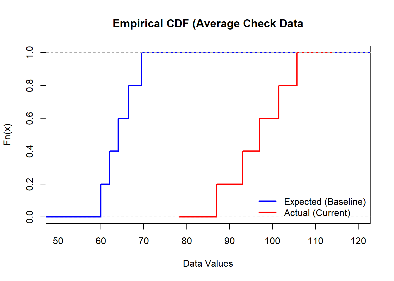
plot(ecdf(expected), col = "blue",
     verticals = TRUE,
     do.points = FALSE,
     main = "Empirical CDF (Average Check Data",
     xlab = "Data Values",
     ylab = "Fn(x)",
     xlim = c(50,120),
     lwd = 2)

plot(ecdf(actual),
     col = "red",
     verticals = TRUE,
     do.points = FALSE,
     add = TRUE, lwd = 2)

legend("bottomright", legend = c("Expected (Baseline)", "Actual (Current)"),
       col = c("blue", "red"), lwd = 2, bty = "n")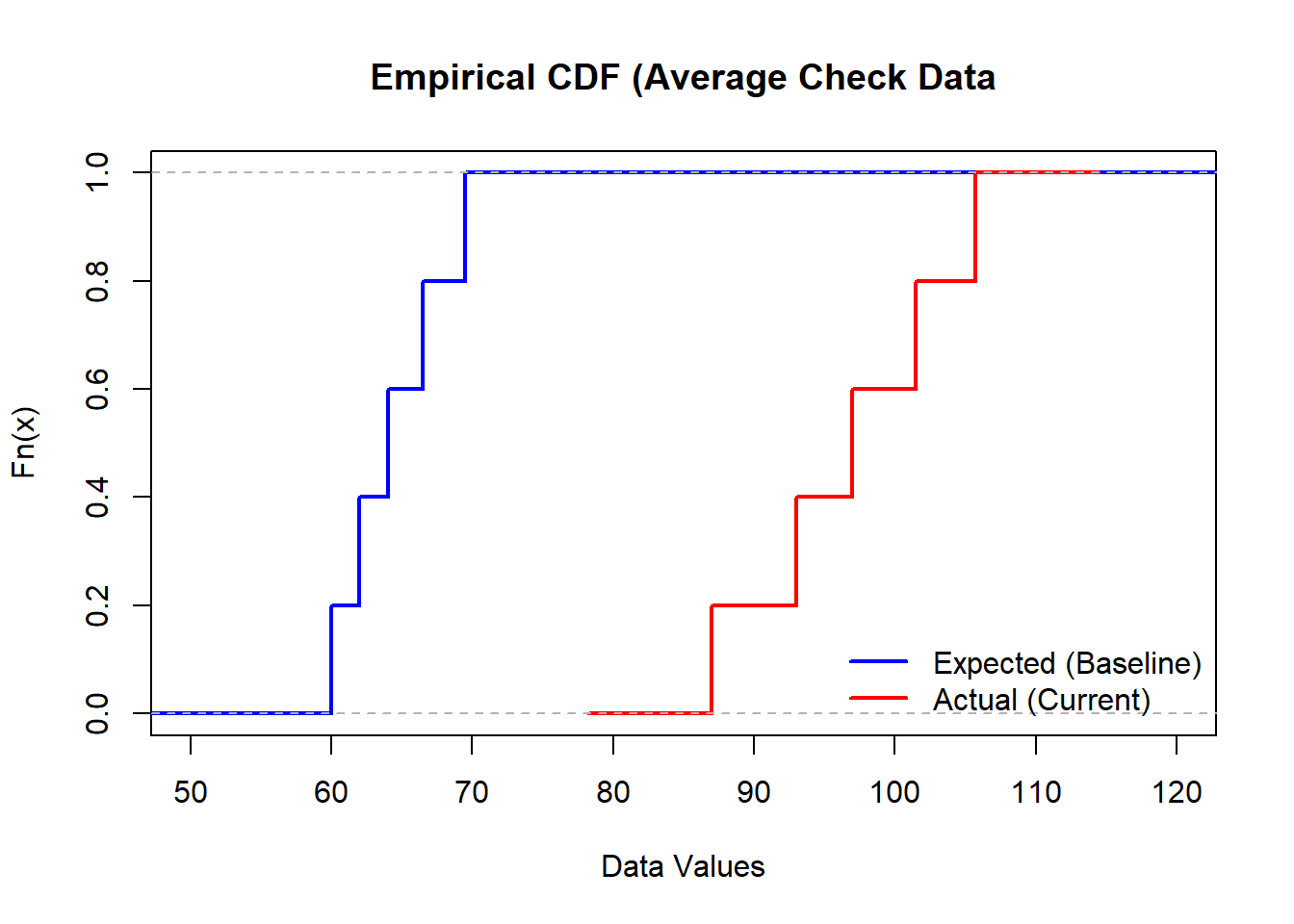
Here is a better quality ggplot.
df_baseline <- data.frame(Value = expected,
                          Dataset = "expected")

df_target   <- data.frame(Value = actual,
                          Dataset = "actual")

plot_data   <- rbind.data.frame(df_baseline, df_target)


ggplot(plot_data, aes(x = Value, color = Dataset)) +
  stat_ecdf(geom = "step", linewidth = 1) +

  labs(
    title = "Hoboken Fine Dining Average Check Data",
    subtitle = "eCDF Drift Comparison",
    x = "Dollars ($)",
    y = "Cumulative Proportion"
  ) +
  theme_minimal(base_size = 14) +
  theme(legend.position = "bottom")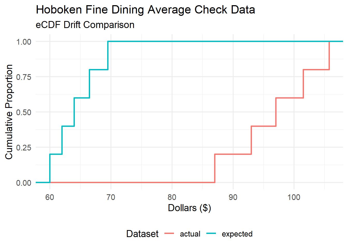
Visually, the data suggests considerable drift, corroborated by the boostrapped results of the KS test. Plaintiff’s expert cannot claim that the proffered model’s projections represents a plausible counterfactual.
What were the reasons behind the data drift?
Key Trends & Cost Drivers entail (i) menu inflation; (ii) changing consumer habits; and, (iii) local business pressures.
Menu Inflation: From 2020 to 2025, chain restaurant pricing increased by an average of $42 nationally, and local dining spots in Hoboken mirrored this trend. Micro-indicators show that regular items like cold brews and burgers rose by 3% to 4.5%.
Changing Consumer Habits: Because the local median household income is high (hovering around $180,000, diners still frequent upscale spots like Del Frisco’s Grille and Augustino’s. However, to offset higher check averages elsewhere, patrons increasingly seek out loyalty perks, happy hours, and value-driven promotions.
Local Business Pressures: Many popular Hoboken establishments attributed recent, drastic price jumps to severe overhead challenges, including high rent renewals and rising property values along the waterfront.
This may not be a silver stake but it certainly raises credible and powerful questions as to the soundness of plaintiff’s work.